Estimate the FARMA operators

Estimates the operators of a FARMA(p, q) model by the functional Hannan-Rissanen method of Kuenzer (2024). The curves are assumed to be short-memory, so long-memory curves need to be fractionally differenced first, for example with frac_diff(). farfima() does this on the centred training curves and drops the first trim before estimating the operators.

Usage

estimate_operators(x, order, Npc = 1)

# S3 method for class 'farfima_operators'
plot(
  x,
  argvals = NULL,
  xlab = "Grid point v",
  ylab = "Grid point u",
  main = NULL,
  ...
)

Arguments

x: A matrix of short-memory curves (grid points by time) or an fts object. For plot(), a farfima_operators object.
order: FARMA orders c(p, q), or a result of select_order().
Npc: Number of principal components in the dimension reduction of the Hannan-Rissanen method.
argvals: Grid values. Defaults to the row names of the curves if numeric.
xlab, ylab, main: Axis labels and title.
...: Other arguments passed to graphics::image().

Value

An object of class farfima_operators with order, the AR and MA operators phi and theta (grid by grid by lag, NULL when the order is zero), and the one-step-ahead in-sample fitted curves and residuals. Printing it shows the norm of each operator.

Details

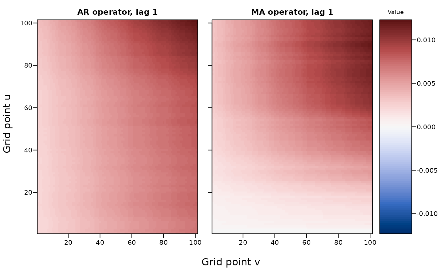
Each operator is stored as a grid by grid matrix, the kernel times the grid spacing, so that applying the operator to a curve is a matrix product. plot() draws the operators as heatmaps, red for positive and blue for negative values.

The estimation code is adapted from code by Thomas Kuenzer.

References

Kuenzer, T. (2024). Estimation of functional ARMA models. Bernoulli.

Examples

x = sim_farfima(n = 300, d = 0, p = 1, q = 1, seed = 1)
op = estimate_operators(x, order = c(1, 1))
op
#> FARMA(1, 1) operators
#>   Data:      101 grid points x 300 curves
#>   Operators: functional Hannan-Rissanen estimator with 1 principal component
#>   Norms:     AR lag 1 = 0.623, MA lag 1 = 0.599
plot(op)