farfima: Order Selection and Forecasting in Long-Memory Functional Time Series

Fits FARFIMA models to long-memory functional time series, selects their orders and forecasts the curves with conformal prediction bands. Curves are stored as a matrix with grid points in rows and time in columns. fts objects from rainbow and ftsa also work.

Workflow

split_curves() splits the curves into training, validation and test samples, and plot_curves() draws them.
farfima() fits the model. It estimates the memory parameter with estimate_memory(), selects the FARMA orders of the fractionally differenced curves as in select_order(), estimates their operators as in estimate_operators(), and calibrates the conformal prediction bands on the validation sample. fitted() and residuals() give the in-sample fit, and plot() draws it.
predict() forecasts from the fit, with conformal prediction bands, and evaluates the forecasts on a test sample.
plot() visualises the forecasts, and as.data.frame() puts them in a table.

Other functions

estimate_memory(), select_order() and estimate_operators(): the steps of farfima(), which can also be run on their own. select_order() and estimate_operators() take short-memory curves, such as fractionally differenced curves.
frac_diff(): fractional differencing.
sim_farfima(): simulated long-memory functional time series.

Author

Chang Liu, Han Lin Shang, Garth Tarr and Samuel Müller. Maintainer: Chang Liu chang.liu45@students.mq.edu.au

Examples

sim = sim_farfima(n = 200, d = 0.3, p = 1, q = 1, no_grid = 51, seed = 1)
blocks = split_curves(sim, train = 0.6, valid = 0.2)
fit = farfima(blocks$train, blocks$valid, d = "lpwn2", order = "ic_full",
               p = 0:2, q = 0:2, h = 5, trim = 30)
#> Selecting (p, q) by functional IC over 8 candidates
#> Calibrating the SR, NS, AC bands on 40 validation origins (36 at h = 5)
fc = predict(fit, test = blocks$test, band = "AC")
#> Evaluating on 40 test origins
fc
#> Forecasts from FARFIMA(p = 1, d = 0.3084, q = 0)
#>   Horizons:  h = 1..5 after curve 200 (expanding window)
#>   Bands:     AC (adaptive conformal)
#>   Levels:    80%, 95%
#> 
#> Test evaluation over 40 test curves, averaged over horizons:
#>   RMSPE = 1.135, MAPE = 0.8865
#>  band level    ECP     CPD   MIS
#>    AC   80% 0.7522 0.04780 3.867
#>    AC   95% 0.9173 0.03271 5.485
#>   WIS: AC = 0.3868
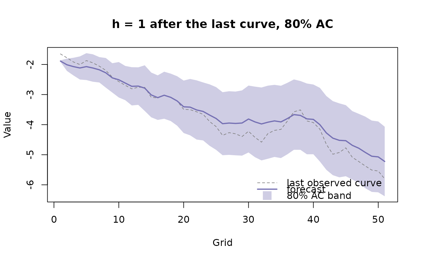
plot(fc, h = 1)

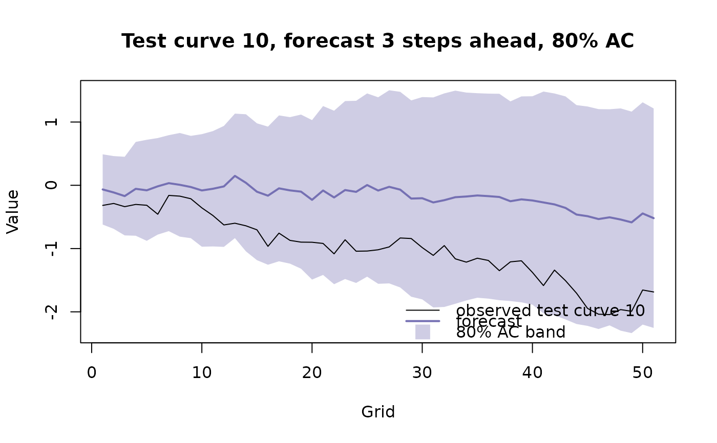
plot(fc, h = 3, target_test_curve = 10)